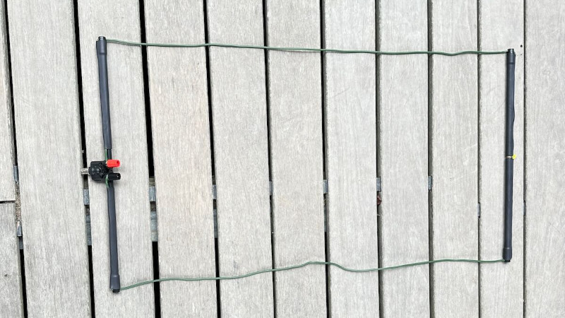
One of amateur radio’s many interests comes in portable operation, taking your radio to an out of the way place, usually a summit, and working the world using only what can be carried in. Often this means using the HF or shortwave bands, but the higher frequencies get a look-in as well. A smaller antenna is no less the challenge when it comes to designing one that can be carried though, and [Thomas Witherspoon] demonstrates this with a foldable loop antenna for the 2 metre band.
The antenna provides a reminder that the higher bands are nothing to be scared of in construction terms, it uses a BNC-to-4 mm socket adapter as its feedpoint, and makes the rectangular shape of the loop with pieces of fiberglass tube. The wire itself is flexible antenna wire, though we’re guessing almost any conductor could be used. The result is a basic but useful antenna that certainly packs down to a very small size, and we can see it would be a useful addition to any portable operator’s arsenal.
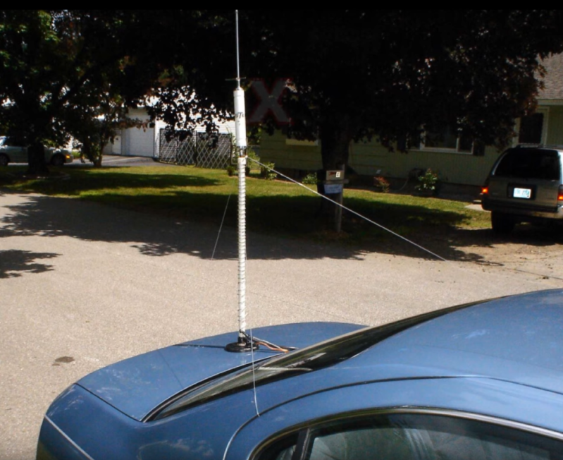
The real action in the world of ham radio is generally in the high frequency bands. Despite the name, these are relatively low-frequency bands by modern standards and the antenna sizes can get a little extreme. After all, not everyone can put up an 80-meter dipole, but ham radio operators have come up with a number of interesting ways of getting on the air anyway. The only problem is that a lot of these antennas don’t seem as though they should work half as well as they do, and [MIKROWAVE1] takes a look back on some of the more exotic radiators.
He does note that for a new ham radio operator it’s best to keep it simple, beginning work with a dipole, but there are still a number of options to keep the size down. A few examples are given using helically-wound vertical antennas or antennas with tuned sections of coaxial cable. From there the more esoteric antennas are explored, such as underground antennas, complex loops and other ways of making a long wire fit in a small space, and even simpler designs like throwing a weight with a piece of wire attached out the window of an apartment building.
While antenna theory is certainly a good start for building antennas, a lot of the design of antennas strays into artistry and even folklore as various hams will have successes with certain types and others won’t. It’s not a one-size-fits-all situation so the important thing is to keep experimenting and try anything that comes to mind as long as it helps get on the air. A good starting point is [Dan Maloney]’s $50 Ham Guide series, and one piece specifically dealing with HF antennas.
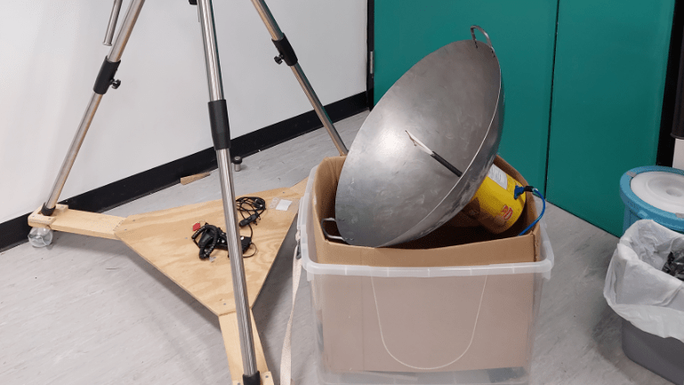
The round bottom of a proper wok is the key to a decent stir fry, but it also makes it hard to use on traditional Western stoves. That’s why many woks end up in a dark kitchen cabinet, unused and unloved. But wait; it turns out that the round bottom of a wok is the perfect shape for gathering something else — radio waves, specifically the 21-cm neutral hydrogen emissions coming from the heart of our galaxy.
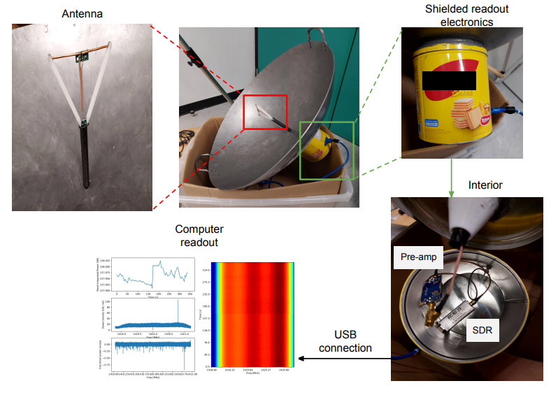
Turning a wok into an entry-level radio telescope doesn’t appear to be all that hard, at least judging by what [Leo W.H. Fung] et al detail in their paper (PDF) on “WTH” or “Wok the Hydrogen.” Aside from the wok, which serves as the main reflector, you’ll need a bit of coaxial cable and some stiff copper wire to fashion a small dipole antenna and balun, plus some plastic tubing to support it at the focal point of the reflector. Measuring the wok’s shape and size, which in turn determines its focal point, is probably the hardest part of the build; luckily, the paper includes tips on doing just that. The authors address the controversy of parabolic versus spherical reflectors and arrive at the conclusion that for a radio telescope fashioned from a wok, it just doesn’t matter.
As for the signal processing chain, WTH holds few surprises. A Nooelec Sawbird+ H1 acts as preamp and filter for the 1420-MHz hydrogen line signal, which feeds into an RTL-SDR dongle. Careful attention is paid to proper grounding and shielding to keep the noise floor as low as possible. Mounting the antenna is a decidedly ad hoc affair, and aiming is as simple as eyeballing various stars near the center of the galactic plane — no need to complicate things.
Performance is pretty good: WTH measured the recession velocity of neutral hydrogen to within 20 km/s, which isn’t bad for something cobbled together from scrap. We’ve seen plenty of DIY hydrogen line observatories before, but WTH probably wins the “get on the air tonight” award.
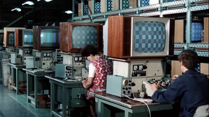
For those of us who lived through the Cold War, there’s still an air of mystery as to what it was like on the Communist side. As Uncle Sam’s F-111s cruised slowly in to land above our heads in our sleepy Oxfordshire village it was at the same time very real and immediate, yet also distant. Other than being told how fortunate we were to be capitalists while those on the communist side lived lives of mindless drudgery under their authoritarian boot heel, we knew nothing of the people on the other side of the Wall, and God knows what they were told about us. It’s thus interesting on more than one level to find a promotional film from the mid 1970s showcasing VEB Fernsehgerätewerk Stassfurt (German, Anglophones will need to enable subtitle translation), the factory which produced televisions for East Germans. It provides a pretty comprehensive look at how a 1970s TV set was made, gives us a gateway into the East German consumer electronics business as a whole, and a chance to see how the East Germany preferred to see itself.
The RFT range of televisions in the Städtisches Kaufhaus exhibition center for the 1968 Leipzig Spring Fair. Bundesarchiv, CC-BY-SA 3.0
The sets in question are not too dissimilar to those you would have found from comparable west European manufacturers in the same period, though maybe a few things such as the use of a tube output stage and the lack of integrated circuits hints at their being a few years behind the latest from the likes of Philips or ITT by 1975. The circuit boards are assembled onto a metal chassis which would have probably been “live” as the set would have derived its power supply by rectifying the mains directly, and we follow the production chain as they are thoroughly checked, aligned, and tested. This plant produces both colour and back-and-white receivers, and since most of what we see appears to be from the black-and-white production we’re guessing that here’s the main difference between East and West’s TV consumers in the mid ’70s.
The film is at pains to talk about the factory as a part of the idealised community of a socialist state, and we’re given a tour of the workers’ facilities to a backdrop of some choice pieces of music. References to the collective and some of the Communist apparatus abound, and finally we’re shown the factory’s Order of Karl Marx. As far as it goes then we Westerners finally get to see the lives of each genosse, but only through an authorised lens.
The TVs made at Stassfurt were sold under the RFT East German technology combine brand, and the factory continued in operation through the period of German re-unification. Given that many former East German businesses collapsed with the fall of the Wall, and that the European consumer electronics industry all but imploded in the period following the 1990s then, it’s something of a surprise to find that it survives today, albeit in a much reduced form. The plant is now owned by the German company TechniSat, and manufactures the latest-spec digital TVs. Meanwhile for those interested in history there’s a museum exhibition in the town (German language, Google Translate link), which looks very much worth a visit should you be motoring across Germany.
As degenerate capitalists we weren’t offered the privilege of buying a TV from the Worker’s Paradise, so we never had the opportunity to see how their quality stacked up to that of the Western models. It’s worth remembering that however rose-tinted our view of the 1970s may be, British-made sets of the period weren’t particularly reliable themselves.
Anybody who has set up a satellite TV antenna will tell you that alignment is critical when picking up a signal from space. With a satellite dish it’s a straightforward task to tweak the position, but what happens if the dish in question is out beyond the edge of the Solar System?
We told you a few days ago about this exact issue currently facing Voyager 2, but we’re guessing Hackaday readers will want to know a little bit more about how a 50+ year old spacecraft so far from home can still sort out its antenna. The answer lies in NASA Technical Report 32-1559, Digital Canopus Tracker from 1972, which describes the instrument that notes the position of the star Canopus, which along with that of the Sun it can use to calculate the antenna bearing to reach Earth. The report makes for fascinating reading, as it describes how early-1970s technology was used to spot the star by its specific intensity and then keep it in its sights. It’s an extremely accessible design, as even the part numbers are an older version of the familiar 74 logic.
So somewhere out there in interstellar space beyond the boundary of the Solar System is a card frame full of 74 logic that’s been quietly keeping an eye on a star since the early 1970s, and the engineers from those far-off days at JPL are about to save the bacon of the current generation at NASA with their work. We hope that there are some old guys in Pasadena right now with a spring in their step.
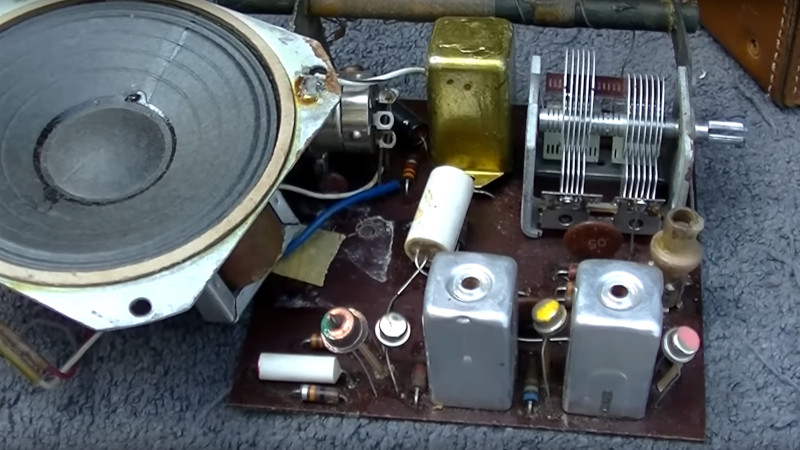
Here in 2023 the field of electronics covers a breathtaking variety of devices and applications, but if we were to go back in time far enough we’d enter an age in which computers were few and far between, and any automated control systems would have been electromechanical at best. Back in the 1950s the semiconductor industry was in relative infancy, and at the consumer end electronics were largely synonymous with radio. [Shango066] brings us a transistor radio from that era, a Jewel TR1 from about 1958, that despite its four-transistor simplicity to our eyes would have been a rare and expensive device when new.
As you’d expect, a transistor radio heading toward its 70th birthday requires a little care to return to its former glory, and while this one is very quiet it does at least work after a fashion. The video below the break is a long one that you might wish to watch at double speed, but it takes us through the now-rare skill of fault-finding and aligning an AM radio receiver. First up are a set of very tired electrolytic capacitors whose replacement restores the volume, and then it’s clear from the lack of stations that the set has a problem at the RF end. We’re treated to the full process of aligning a superhet receiver through the relatively forgiving low-frequency medium of a medium-wave radio. Along the way, he damages one of the IF transformers and has to replace it with a modern equivalent, which we would have concealed under the can from the original.
The video may be long, but it’s worth a look for the vintage parts if not for the quality of radio stations on the air today in California. For many readers, AM broadcast is becoming a thing of the past, so we’re not sure we’ll see this very often.
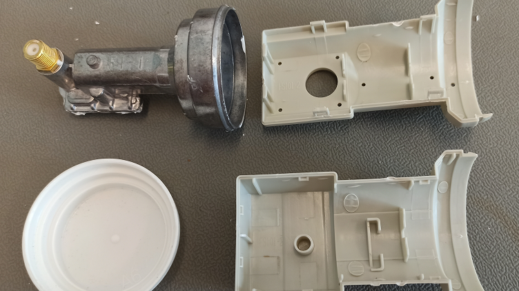
A word of advice: If you see an old direct satellite TV dish put out to the curb, grab it before the trash collector does. Like microwave ovens, satellite dishes are an e-waste wonderland, and just throwing them away before taking out the good stuff would be a shame. And with dishes, the good stuff basically amounts to the bit at the end of the arm that contains the feedhorn and low-noise block downconverter (LNB).
But what does one do with such a thing once it’s harvested? Lots of stuff, including modifying it for use with the QO-100 geosynchronous satellite. That’s what [Sebastian Westerhold] and [Celin Matlinski] did with a commodity LNB, although it seems more like something scored on the cheap from one of the usual sources rather than picking through trash. Either way, these LNBs are highly integrated devices that at built specifically for satellite TV use, but with just a little persuasion can be nudged into the K-band to receive the downlink signals from hams using QO-100 as a repeater.
The mods are simple — snipping out the 25 MHz reference crystal on the LNB board and replacing it with a simple LC bandpass filter. This allows the local oscillator on the LNB to be referenced to an external signal generator; when fed with a 25.78 MHz signal, it’s enough to goose the LNB up to 10,490 MHz — right about the downlink frequency. [Sebastian] and [Celin] tested the mods and found that it was easily able to detect the third harmonics of a 3.5-ish GHz signal.
As for testing on actual downlink signals from the satellite, that’ll have to wait. For now, if you’re interested in satellite comms, and you live on the third of the planet covered by QO-100, keep an eye out for those e-waste LNBs and get to work.
There was a time when buying a new radio was something many hams could never afford to do. Then came the super cheap — and super controversial — VHF and UHF radios from China. But as they say, you get what you pay for. The often oddly named handhelds like Baofeng and Wouxun are sometimes odd to work with and may have questionable RF outputs. A new radio has a less tongue-twisting English name and many improved features for about $50 — the Talkpod A36Plus and [Josh] shows us how they work in a video that you can see below.
The new features are generally good. For example, the radio can pick up AM in the aircraft band, something most of these cheap radios won’t do. It works on VHF and UHF bands but also picks up FM broadcasts. The USB-C connector is welcome, and the screen is large and colorful. It has 500 channels and IP5 water resistance.
There were a few issues, though. If you want to use it as a scanner, it’s not very fast. The radio comes with a programming cable, but apparently, it uses an odd USB chipset that may give you some driver issues. The biggest problem, though, is that it has, according to the video, excessive spurious emissions. The power isn’t that high, and the antenna probably filters off some of it, too. But creating interference across the band isn’t very polite.
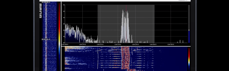
How bad are the harmonics? Well, [Josh] hooks up a spectrum analyzer and also shows how a radio tuned to the second harmonic easily picks up the transmission. Of course, no radio is perfect, but it seems like it does have very strong harmonic emissions. Of course, it may or may not be any worse than similar cheap radios. They are probably all above the legal limits, and it is just a matter of degrees.
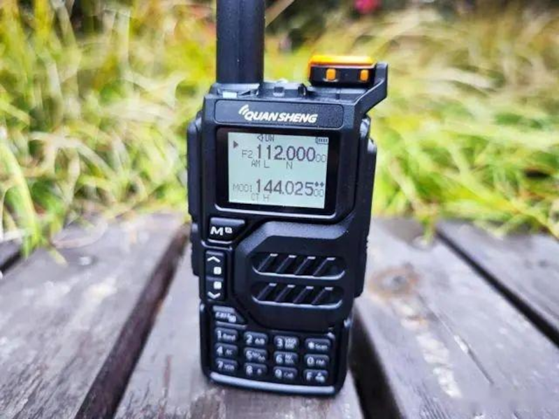
Over the past decade or so, amateur radio operators have benefited from an influx of inexpensive radios based around a much simpler design than what was typically commercially available, bringing the price of handheld dual-band or GMRS radios to around $20. This makes the hobby much more accessible, but they have generated some controversy as they tend to not perform as well and can generate spurious emissions and other RF interference that a higher quality radio might not create. But one major benefit besides cost is that they’re great for tinkering around, as their simplified design is excellent for modifying. This experimental firmware upgrade changes a lot about this Quansheng model.
With the obligatory warning out of the way that modifying a radio may violate various laws or regulations of some localities, it looks like this modified firmware really expands the capabilities of the radio. The chip that is the basis of the radio, the BK4819, has a frequency range of 18-660 MHz and 840-1300 MHz but not all of these frequencies will be allowed with a standard firmware in order to comply with various regulations. However, there’s typically no technical reason that a radio can’t operate on any arbitrary frequency within this range, so opening up the firmware can add a lot of functionality to a radio that might not otherwise be capable.
Some of the other capabilities this modified firmware opens up is the ability to receive in various other modes, such as FM and AM within the range of allowable frequencies. To take a more deep dive on what this firmware allows be sure to check out the original GitHub project page as well, and if you’re curious as to why these inexpensive radios often run afoul of radio purists and regulators alike, take a look at some of the problems others have had in Europe.
Tuning into a GPS satellite is nothing new. Your phone and your car probably do that multiple times a day. But [dereksgc] has been listening to GPS voice traffic. The traffic originates from COSPAS-SARSAT, which is a decades-old international cooperative of 45 nations and agencies that operates a worldwide search and rescue program. You can watch a video about it below.
Nominally, a person in trouble activates a 406 MHz beacon, and any of the 66 satellites that host COSPAS-SARSAT receivers can pick it up and relay information to the appropriate authorities. These beacons are often attached to aircraft or ships, but there are an increasing number of personal beacons used by campers, hikers, and others who might be in danger and out of reach of a cell phone. The first rescue from this system was in 1982. By 2021, 3,632 people were rescued thanks to the system.
The satellites that listen to the beacon frequencies don’t process the signals. They use a transponder that re-transmits anything it hears on a much higher downlink frequency. These transponders are always payloads on other satellites like navigation or weather satellites. But because the transponder doesn’t care what it hears, it sometimes rebroadcasts signals from things other than beacons. We were unclear if these were rogue radios or radios with spurious emissions in the translator’s input range.
The video has practical tips on how to tune in several of the satellites that carry these transponders. Might be a fun weekend project with a software-defined radio.