QO-100 / Es’hail 2 thuis ontvangen

Op 15 november 2018 werd vanaf Kennedy Spacecenter de Es’hail 2 gelanceerd richting een geostationaire baan om de aarde en sinds enige tijd is de satelliet te gebruiken door radiozendamateurs.

Met een downlink op 10 GHz en een uplink op 2,4 GHz is de satelliet door amateurs betrekkelijk eenvoudig te gebruiken. Het blijkt dat het ontvangen van de satelliet eenvoudiger is dan gedacht. Thijs, PE1RLN neemt je graag mee in zijn ervaringen bij het ontvangen van de smalband communicatie.

10GHz omzetten

Het ontvangen van een 10 GHz signaal lijkt heel moeilijk maar is met behulp van wat hulpmiddelen erg eenvoudig. Elke satellietschotel heeft een LNB (low noise blockconverter) die het 10GHz signaal van bijvoorbeeld de Astra satelliet omlaag brengt naar circa 900 MHz, een frequentie die al beter te behappen is. Maar voor ons radiozendamateurs geen gangbare frequentie natuurlijk.

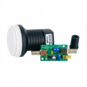
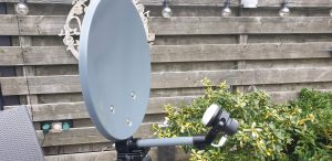
De LNB links op de foto kun je vinden bij Passion Radio en deze transformeert het 10 GHz signaal van de Es’hail naar 432 MHz ! Kijk, dan wordt het interessant.

De LNB is voorzien van een 0,5ppm TCXO voor goede stabiliteit en je krijgt er een bias-tee bij om de LNB te voorzien van spanning. Deze werkt namelijk op 12V via de coax. Bij 12V werkt de LNB op vertikale polarisatie, prima voor de smalband transponder. Bij 14-18V werkt hij horizontaal voor de breedband transponder. Voor € 80 heb je ‘m thuisbezorgd binnen een paar dagen.

De IC-9700 transceiver van Icom kan op de antenne-aansluiting ook 12V tijdens RX afgeven, dan heb je de bias-tee niet nodig.

De lokale oscillator in de LNB werkt op 10.057 MHz dus bijvoorbeeld het PSK baken op 10.489,750 MHz ontvang je straks op 432,750 MHz.

Schotel

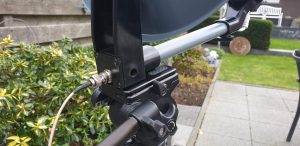
Schotels zijn voor shoarma én om satellieten te ontvangen. Thijs had nog een 35cm campingschotel liggen en die bleek prima te functioneren voor ontvangst! Dus investeer niet in grote radiotelescopen, 35cm volstaat. Zorg dat je een stevig statief hebt want het uitrichten komt een beetje precies.

De LNB wordt voorop gemonteerd en wel zodanig dat deze een “skew” heeft van -15,9 graden. Dat betekent dat de LNB gekanteld wordt met de wijzers van de klok mee als je over de LNB heen naar de schotel kijkt. Dat heeft te maken met de kanteling (skew) van de polarisatie van de satelliet zelf. Hoe beter de skew is afgeregeld, hoe sterker het signaal.

Aansluiten

De LNB en de bias-tee zijn voorzien van F-connectoren, zeer gebruikelijk bij satelliet-TV. Thijs heeft achter op de schotel een BNC aansluiting gemaakt en heeft de bias-tee in een kastje ingebouwd met BNC-connectoren. De impedantie klopt niet helemaal en dat levert verlies op maar de LNB geeft zo’n keihard signaal af dat je dat prima kunt permitteren. Op de bias-tee zit zelfs een attenuator die het signaal dempt en die heb je zeker nodig.

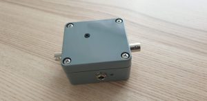
De bias-tee komt dus tussen LNB en ontvanger (tenzij je ontvanger al 12V op de coax heeft) en dan stem je af op 432,750 MHz.

Met het stelknopje in de deksel kun je de attenuation instellen. Aangezien de coax kort is en de LNB een hard signaal geeft, kun je deze best zo instellen dat bij een normale RF gain je waterfall weinig ruis laat zien zodat signalen goed zichtbaar zijn. Dit is handig bij het uitrichten.

Uitrichten van de schotel

Stel de schotel bijna vertikaal en richt de arm van de LNB richting het zuiden. Draai vervolgens 26 graden naar het oosten (tegen wijzers van de klok in dus).

Kijk voor de duidelijkheid op www.dishpointer.com voor precieze uitrichting van je schoteltje. Een schotel met elevatie-gradenboog op de achterkant is ook gemakkelijk om de beginpositie te vinden.

Als je de ontvanger aanzet met een waterfall display dan zie je bij een juiste uitrichting allemaal signalen opdoemen rond 432,750 MHz. Je zult merken dat de afstelling van de schotel niet ultra-precies is maar als je de RF gain terugdraait dan kun je aan de hand van de S-meter de maximale uitslag zoeken met de schotel.

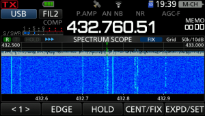
De signalen zijn zeer goed te nemen, alsof het lokale SSB signalen zijn. En dat op een afstand van 35.786 km !!! Had je niet gedacht he?

Je ziet dat de signalen niet heel ver boven de ruis uit komen maar de S/R ratio is prima. De LNB versterkt ook ruis en alleen een grotere schotel maakt het signaal nog schoner. Maar dat levert geen beter signaal op, dit is namelijk al prima.

Luisteren!

Nu kun je met de ontvanger over de hele band draaien, van 432,500 MHz tot 433,000 MHz. Je hoort onderin CW en in het midden de SSB signalen volgens onderstaand bandplan:

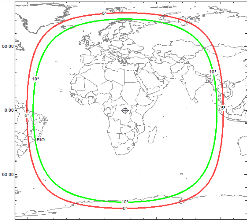
Onderstaand een plot van de dekking van de satelliet:


Welcome To Solar Cycle 25; Our Sun Enters A New 11-Year Period

Most of us perceive time as an arrow, a one-way trip into the future. And while that’s true, nature has a way of interpolating circular patterns onto that linear model — day follows night, the seasons progress through the year, and generations are born, live, and die after creating the next generation to do experience the same cycles in the future.

Our star, too, follows this cyclical model, and goes through observable, periodic changes that are of keen interest to solar scientists. So it was with some fanfare that they recently announced that the sun had transitioned into Solar Cycle 25. But what exactly does that mean? Does the Sun’s changing face make much difference to the average person’s daily life? History shows that it can, so it pays to know what we’re in store for over the next couple of decades. Welcome to your primer on Solar Cycle 25.


It Goes to Eleven

For as long as scientists have had the ability to (safely) observe the Sun, they’ve noticed that our star is not the perfect glowing orb it at first appears to be. Galileo was among the first to observe that the Sun was marked by small dark imperfections. Observers began to keep track of these sunspots, noting not only their variable number but the fact that they migrate across the Sun’s surface with time.

It would take almost two and a half centuries for anyone to notice that the periodic nature of the patterns of sunspots. German scientist Samuel Heinrich Schwabe is credited with the discovery of the solar cycle in 1843 after 17 years of observations of the average number of sunspots. Swiss scientists Rudolf Wolf used the observations of Schwabe and others to backtrack through the data back to 1755. For solar science purposes, this was designated the year that Solar Cycle 1 started.

Cycles of sunspots for the last 400 years. The earliest data is estimated from geological and tree-ring records. By Robert A. Rohde, CC BY-SA 3.0

The cycle these pioneering solar scientists had discovered has a remarkably regular eleven-year period. The range of variation is very tight, from the nine-year period of Solar Cycle 2 (1766 to 1775) to almost fourteen years for Solar Cycle 4 (1784 to 1798). Each solar cycle is reckoned from a solar minimum, essentially when the sunspot number reaches its local low. The number of sunspots increases over the first half of the cycle, peaking at the solar maximum point before turning down again to head for the next solar minimum.

The raw number of sunspots is not the only interesting cycle the Sun displays. The distribution of sunspots across the Sun’s surface also changes periodically with the solar cycle. At the beginning of each solar cycle, what few sunspots there are tend to cluster at the Sun’s equator. As the cycle progresses and the Sun becomes more active, the sunspots tend to pop up further away from the equator, generally clustering around the mid-latitudes around 30° north and south. As solar maximum passes, sunspots again migrate back to the equator to start the cycle again.

Flipping Magnetic Poles

The periodic changes in the number and distribution of sunspots may be an interesting observation, but what does it mean here on Earth? To help understand that, it pays to recall that despite their dark appearance, sunspots are only marginally cooler than the surrounding solar material. Sunspots are still extremely energetic areas, and as the number of sunspots increases, the output of the Sun (in terms of luminosity) increases.

Sunspots represent places where concentrated lines of magnetic force emerge from deep within the Sun’s interior. Thus a change in the number and location of sunspots reveals changes in the magnetic field of the Sun. It turns out that what’s behind the solar cycle is these periodic changes in the Sun’s magnetic field. (It’s important to note here that the eleven-year cycle is technically the “sunspot cycle,” and the 22-year pole-flipping cycle is the true “solar cycle,” but it’s common practice to use “Solar Cycle” for both.)

The magnetic poles of the Sun are constantly in motion, with the north and south poles flipping every eleven years. At solar minimum, the magnetic poles are roughly aligned with the Sun’s orbital axis, and magnetic lines of force tend to penetrate the photosphere near the equator. As the poles rotate towards the equator, magnetic activity picks up, magnetic lines of force move to high latitudes, increasing the number of sunspots there. The process continues for the back half of the solar cycle as the poles complete their reversal.

So, as each solar cycle progresses due to the migration of the Sun’s magnetic field, solar output increases. Fractional though these changes are, they have obvious implications for life on Earth. But the increasing brightness of our Sun is far from the only impact felt here. The changing magnetic field of the Sun can also have a huge impact on our planet.

What Happens Next?

It’s well known that increased sunspots are associated with stronger and more frequent coronal mass ejections, or CMEs. These events, sometimes energetic in the extreme, occur when magnetic domains in the Sun become so twisted and contorted that they erupt outward, picking up gigatons of highly excited plasma from the Sun’s corona. If the CME occurs in just the right spot on the Sun’s surface, the violently ejected tangle of magnetic flux and plasma can strike the Earth, causing anything from an increase in auroral displays to the catastrophic destruction of infrastructure.

While destructive CMEs are more likely to occur during solar maxima — the 1859 Carrington Event occured near the peak of Solar Cycle 10, and the 1989 Hydro-Québec disaster was about seven months before the peak of Solar Cycle 22 — it’s far from a rule that they only occur then. Plenty of damaging or potentially dangerous CMEs have occurred during solar minima. But the number of CMEs goes up dramatically with the sunspot number, so that the Sun launches a few large outbursts each day during a solar maximum. Simply increasing the number of shots increases the chances of a devasting strike.

While the increased risk of Earth-striking CMEs during solar maximum is a concern, it’s important to keep in mind a few things. First, solar maximum is still about five years away; NASA says that Solar Cycle 25 officially began in December of 2019, meaning we’re still very much in solar minimum conditions. Second, not all solar cycles are created equal. Layered on top of the eleven-year solar cycle are other periodic cycles that we’re only beginning to understand. One is the Gleissberg Cycle, an 87-ish-year cycle where the solar maxima of the eleven-year cycle tend to increase and decrease. We’re currently in the decreasing phase of the Gleissberg Cycle, meaning that the just-completed Solar Cycle 24 had a much lower solar maximum than the previous cycle. The current prediction is that Solar Cycle 25 will be about the same intensity as the previous cycle at solar maximum, and will reach solar maximum around July of 2025.

Source: Space Weather Prediction Center-NOAA

The potential for a sleepy sun for the next eleven years is a “good news, bad news” thing. On the plus side, there’s a greatly reduced — but far from zero — risk of experiencing a catastrophic Earth-striking CME. That means less risk to our vulnerable infrastructure, both terrestrial in terms of the millions of miles of power and communications wires we’ve stitched together, and space-based, since satellites can be greatly impacted by space weather. On the other hand, amateur radio operators and others who depend on ionospheric skip for long-range radio communications, like marine operators, airlines, and the military, always get grumpy when the sun is less active, since fewer sunspots mean decreased ionization of Earth’s atmosphere.

In the end, the Sun is going to do what it does, regardless of how it impacts life here on Earth. All we can do is learn everything possible about the star at the center of our solar system, build good models to predict its behavior over time, and build systems that can withstand our star’s mood swings.

P

M17 Aims To Replace Proprietary Ham Radio Protocols

While M17 might sound like a new kind of automatic rifle (as actually, it is), we were referring to an open source project to create a ham radio transceiver. Instead of paraphrasing the project’s goals, we’ll simply quote them:

The goal here should be to kick the proprietary protocols off the airwaves, replace DMR, Fusion, D-Star, etc. To do that, it’s not just good enough to be open, it has to be legitimately competitive.

Like some other commercial protocols, M17 uses 4FSK along with error correction. The protocol allows for encryption, streaming, and the encoding of callsigns in messages. There are also provisions for framing IP packets to carry data. The protocol can handle voice and data in a point-to-point or broadcast topology.


On the hardware side, the TR-9 is a UHF handheld that can do FM voice or M17 with up to 3 watts out. The RF portion uses an ADF7021 chip which is specifically made to do 4FSK. There’s also an Arm CPU to handle the digital work.

We were struck by the similarity of the TR-9 to a cell phone since it has an LCD display, an SD card slot, and a 9DOF sensor.  Maybe some open hardware cell phones and open hardware ham radios could find common ground.

This is quite ambitious, but generally, small ham rigs are having a resurgence. Having high-quality RF components available as chips makes a lot of difference.

P