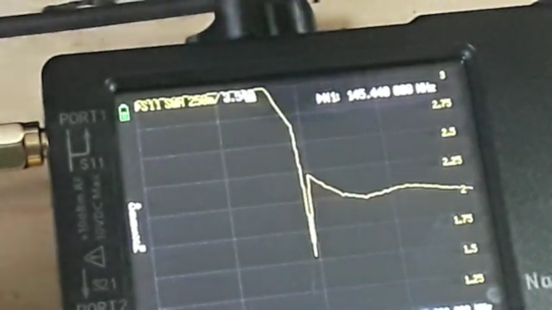
When you buy a cheap ham radio handy-talkie, you usually get a little “rubber ducky” antenna with it. You can also buy many replacement ones that are at least longer. But how good are they? [Learnelectronics] wanted to know, too, so he broke out his NanoVNA and found out that they were all bad, although some were worse than others. You can see the results in the — sometimes fuzzy — video below.
Of course, bad is in the eye of the beholder and you probably suspected that most of them weren’t super great, but they do seem especially bad. So much so, that, at first, he suspected he was doing something wrong. The SWR was high all across the bands the antennas targeted.
It won’t come as a surprise to find that making an antenna work at 2 meters and 70 centimeters probably isn’t that easy. In addition, it is hard to imagine the little stubby antenna the size of your thumb could work well no matter what. Still, you’d think at least the longer antennas would be a little better.
Hams have had SWR meters for years, of course. But it sure is handy to be able to connect an antenna and see its performance over a wide band of frequencies. Some of the antennas weren’t bad on the UHF band. That makes sense because the antenna is physically larger but at VHF the size didn’t seem a big difference.
He even showed up a little real-world testing and, as you might predict, the test results did not lie. However, only the smallest antenna was totally unable to hit the local repeater.
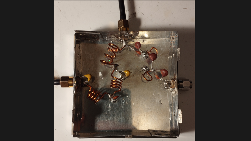
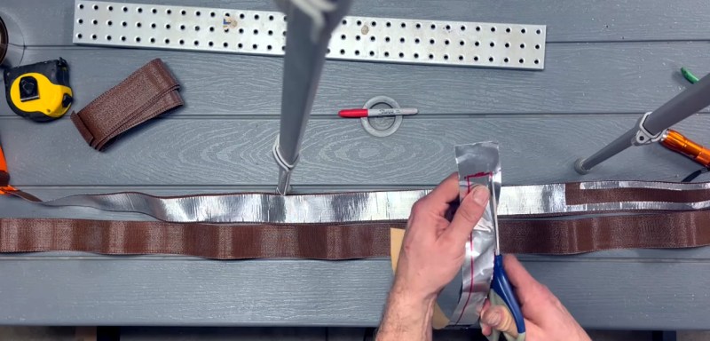
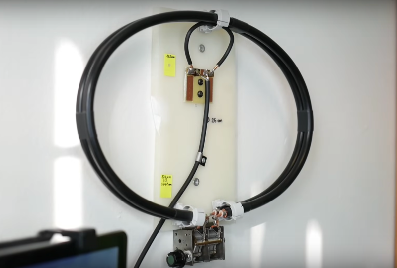
Of course, you can always make your own antenna. It doesn’t have to take much.