Analog radio broadcasts are pretty simple, right? Tune into a given frequency on the AM or FM bands, and what you hear is what you get. Or at least, that used to be the way, before smart engineers started figuring out all kinds of sneaky ways for extra signals to hop on to mainstream broadcasts.
Subcarrier radio once felt like the secret backchannel of the airwaves. Long before Wi-Fi, streaming, and digital multiplexing, these hidden signals beamed anything from elevator music and stock tickers to specialized content for medical professionals. Tuning into your favorite FM stations, you’d never notice them—unless you had the right hardware and a bit of know-how.
Sub-what now?
Subcarrier radio was approved by the FCC under the Subsidiary Communications Authorization. This allowed both AM and FM radio stations to deliver additional content through subchannel broadcasting on their existing designated frequency. Practicalities mean that only FM stations could reasonably use this technique to broadcast additional audio content; AM radio stations were too limited in bandwidth to do so. In the latter case, only low-bitrate data could be sent on a subcarrier. 1983 saw the deregulation of subcarrier broadcasts, with existing broadcasters able to use them largely as they wished.
To understand how this let FM radios broadcast extra programming, we need to know how subcarriers work. Basically, in this context, a subcarrier is a high-frequency signal outside the range of human hearing—usually something like a sine wave at a frequency of 20 KHz to 100 KHz or so. This signal is then amplitude modulated with the desired secondary audio program for broadcast. As this signal is beyond the range of human hearing, it can be mixed with the regular station’s main audio feed without perceptibly altering it to any great degree. The mixed signal is then frequency modulated on to the radio station’s main carrier signal (usually in the range of 88-108 MHz) and sent up the tower for broadcast over radio.
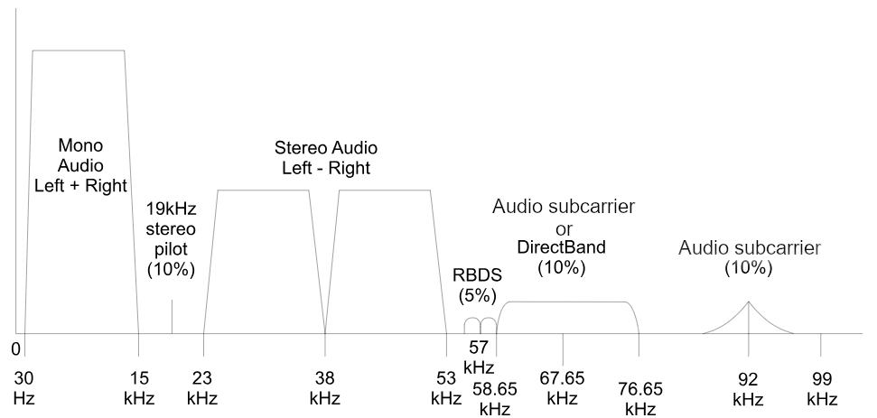
For subchannel broadcasting, FM stations typically used subcarriers at 67 kHz or 92 kHz to carry additional low-fidelity mono audio feeds. These carrier frequencies were chosen to avoid the existing subcarrier signal in FM stereo broadcasts, which carried a left-right channel difference signal at 38 kHz.
Subcarriers were a neat little lifehack that let a single frequency do double or triple duty. A single FM station could deliver its main program, plus a bonus low-fidelity mono channel for various purposes. This facility was used for all kinds of obscure uses. Some broadcasters delivered background music for piping into department stores and the like, while others created special channels reserved for reading-for-the-blind organizations.
The Physician’s Radio Network was also a notable user, which broadcast information of specific relevance to medical professionals. However, the limited audience made it a difficult prospect to keep running from a commercial standpoint, even though it saved money by merely rebroadcasting one hour of programming around the clock on any given day. It eventually went off the air in 1981.
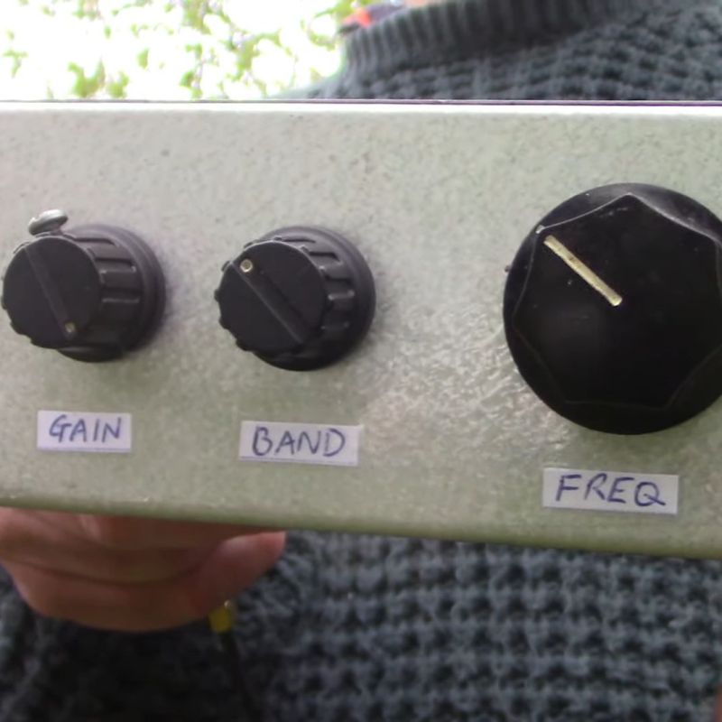
Tuning into these broadcasts wasn’t possible on a regular FM radio. Instead, you needed a device specifically built to pull the subcarrier signal out of the radio broadcast and then demodulate it back into listenable audio. By and large, organizations broadcasting on subchannels would distribute special radios that were tuned to only decode their sub-carrier station. The hardware involved wasn’t complex—it just involved demodulating the FM broadcast signal, then filtering out the subcarrier signal and demodulating that back into audio.

FM subcarriers weren’t just for audio, either. Microsoft famously used 67.7 kHz subcarriers on FM radio stations for its now-defunct DirectBand datacast network. It could deliver data at 12 kbit/second, or over 100 MB a day. The technology was used to deliver things like weather reports and stock prices to early smartwatches and coffee makers in the days before WiFi and celluar internet were cheap and everywhere.
From a hardware hacker’s perspective, these channels were a fun challenge to hunt down. With the right radio receiver and a bit of circuit hacking to tap off the baseband signal, you could decode the subcarrier and reveal the hidden broadcast. Some hobbyists rigged up surplus SCA receivers—often stuff found at flea markets or hamfests—to get free background music, weather reports, or any niche audio that happened to be riding along. Alternatively, decoding the subcarrier was entirely possible by building your own gear. It was kind of a neat analog puzzle—filter out the main audio, isolate the frequency where the secret channel lived, and then demodulate it. The hardware you’d use looked suspiciously like the guts of a standard FM radio, just with a few added filters and demodulation stages stuck in. These days, software defined radio techniques make doing the same thing comparatively easy.
Though it felt like eavesdropping, this wasn’t exactly some top-secret espionage. While technically unauthorized reception was frowned upon by the FCC, it wasn’t heavily policed. Subcarrier channels didn’t exactly have roving gangs of enforcers prowling about the neighborhood. Mostly, these subcarriers delivered paid subscription services, like Muzak, or nonprofit programming authorized under the station’s broadcast license. Their decline coincided with the rise of digital technologies and more flexible content-delivery methods. By the late 20th century, satellite feeds, internet streaming, and multicast digital channels rendered analog subcarriers quaint and unnecessary.
Still, SCA subcarrier signals remain a fascinating piece of broadcasting history. A few still linger today, but it’s now a more obscure medium than ever, lost as mainstream technology has moved on. It’s a reminder that even in the old days of broadcast radio, clever engineers found ways to pack more data into the same old bandwidth—long before we started streaming everything in sight.
Featured image by [windytan]. (Also, check out her work on RDS demodulation.)