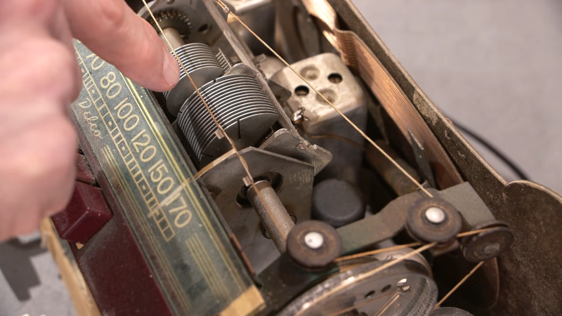
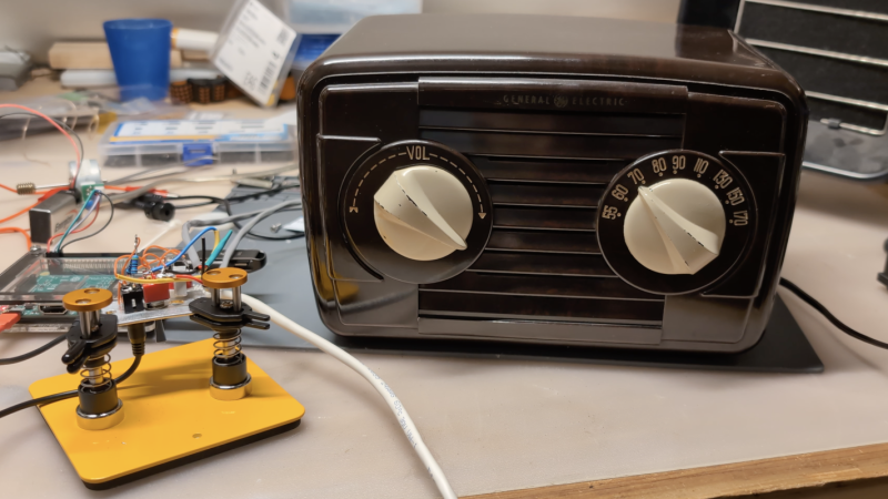
As you might expect, the University of Puerto Rico at Arecibo has a fascination with radio signals from space. While doing research into the legendary “Wow! Signal” detected back in 1977, they realized that the burst was so strong that a small DIY radio telescope would be able to pick it up using modern software-defined radio (SDR) technology.
This realization gave birth to the Wow@Home project, an effort to document both the hardware and software necessary to pick up a Wow! class signal from your own backyard. The University reasons that if they can get a bunch of volunteers to build and operate these radio telescopes, the resulting data could help identify the source of the Wow! Signal — which they believe could be the result of some rare astrophysical event and not the product of Little Green Men.
Ultimately, this isn’t much different from many of the SDR-based homebrew radio telescopes we’ve covered over the years — get a dish, hook your RTL-SDR up to it, add in the appropriate filters and amplifiers, and point it to the sky. Technically, you’re now a radio astronomer. Congratulations. In this case, you don’t even have to figure out how to motorize your dish, as they recommend just pointing the antenna at a fixed position and let the rotation of the Earth to the work — a similar trick to how the legendary Arecibo Observatory itself worked.
The tricky part is collecting and analyzing what’s coming out of the receiver, and that’s where the team at Arecibo hope to make the most headway with their Wow@Home software. It also sounds like that’s where the work still needs to be done. The goal is to have a finished product in Python that can be deployed on the Raspberry Pi, which as an added bonus will “generate a live preview of the data in the style of the original Ohio State SETI project printouts.” Sounds cool to us.
If you’re interested in lending a hand, the team says they’re open to contributions from the community — specifically from those with experience RFI shielding, software GUIs, and general software development. We love seeing citizen science, so hopefully this project finds the assistance and the community it needs to flourish.
For the most part, the Radio Apocalypse series has focused on the radio systems developed during the early days of the atomic age to ensure that Armageddon would be as orderly an affair as possible. From systems that provided backup methods to ensure that launch orders would reach the bombers and missiles, to providing hardened communications systems to allow survivors to coordinate relief and start rebuilding civilization from the ashes, a lot of effort went into getting messages sent.
Strangely, though, the architects of the end of the world put just as much thought into making sure messages didn’t get sent. The electronic village of mid-century America was abuzz with signals, any of which could be abused by enemy forces. CONELRAD, which aimed to prevent enemy bombers from using civilian broadcast signals as navigation aids, is a perfect example of this. But the growth of civil aviation through the period presented a unique challenge, particularly with the radio navigation system built specifically to make air travel as safe and reliable as possible.
Balancing the needs of civil aviation against the possibility that the very infrastructure making it possible could be used as a weapon against the U.S. homeland is the purpose of a plan called Security Control of Air Traffic and Air Navigation Aids, or SCATANA. It’s a plan that cuts across jurisdictions, bringing military, aviation, and communications authorities into the loop for decisions regarding when and how to shut down the entire air traffic system, to sort friend from foe, to give the military room to work, and, perhaps most importantly, to keep enemy aircraft as blind as possible.
Highways in the Sky
As its name suggests, SCATANA has two primary objectives: to restrict the availability of radio navigation aids during emergencies and to clear the airspace over the United States of unauthorized traffic. For safety’s sake, the latter naturally follows the former. By the time the SCATANA rules were promulgated, commercial aviation had become almost entirely dependent on a complex array of beacons and other radio navigation aids. While shutting those aids down to deny their use to enemy bombers was obviously the priority, safety demanded that all the planes currently using those aids had to be grounded as quickly as possible.
The Rogue Valley VOR station in Table Rock, Oregon. According to the sectional charts, this is a VORTAC station. Source: ZabMilenko, CC BY 3.0, via Wikimedia Commons.
Understanding the logic behind SCATANA requires at least a basic insight into these radio navigation aids. The Federal Communications Commission (FCC) has jurisdiction over these aids, listing “VOR/DME, ILS, MLS, LF and HF non-directional beacons” as subject to shutdown in times of emergency. That’s quite a list, and while the technical details of the others are interesting, particularly the Adcock LF beacon system used by pilots to maneuver onto a course until alternating “A” and “N” Morse characters merged into a single tone, but for practical purposes, the one with the most impact on wartime security is the VOR system.
VOR, which stands for “VHF omnidirectional range,” is a global system of short-range beacons used by aircraft to determine their direction of travel. The system dates back to the late 1940s and was extensively built out during the post-war boom in commercial aviation. VOR stations define the “highways in the air” that criss-cross the country; if you’ve ever wondered why the contrails of jet airliners all follow similar paths and why the planes make turns at more or less the same seemingly random point in the sky, it’s because they’re using VOR beacons as waypoints.
In its simplest form, a VOR station consists of an omnidirectional antenna transmitting at an assigned frequency between 108 MHz and 117.95 MHz, hence the “VHF” designation. The frequency of each VOR station is noted on the sectional charts pilots use for navigation, along with the three-letter station identifier, which is transmitted by the station in Morse so pilots can verify which station their cockpit VOR equipment is tuned to.
Each VOR station encodes azimuth information by the phase difference between two synchronized 30 Hz signals modulated onto the carrier, a reference signal and a variable signal. In conventional VOR, the amplitude-modulated variable signal is generated by a rotating directional antenna transmitting a signal in-phase with the reference signal. By aligning the reference signal with magnetic north, the phase angle between the FM reference and AM variable signals corresponds to the compass angle of the aircraft relative to the VOR station.
More modern Doppler VORs, or DVORs, use a ring of antennas to electronically create the reference and variable signals, rather than mechanically rotating the antenna. VOR stations are often colocated with other radio navigation aids, such as distance measuring equipment (DME), which measures the propagation delay between the ground station and the aircraft to determine the distance between them, or TACAN, a tactical air navigation system first developed by the military to provide bearing and distance information. When a VOR and TACAN stations are colocated, the station is referred to as a VORTAC.
Shutting It All Down
At its peak, the VOR network around the United States numbered almost 1,000 stations. That number is on the decrease now, thanks to the FAA’s Minimum Operational Network plan, which seeks to retire all but 580 VOR stations in favor of cockpit GPS receivers. But any number of stations sweeping out fully analog, unencrypted signals on well-known frequencies would be a bonanza of navigational information to enemy airplanes, which is why the SCATANA plan provides specific procedures to be followed to shut the whole thing down.
Inside the FAA’s Washington DC ARTCC, which played a major role in implementing SCATANA on 9/11. Source: Federal Aviation Administration, public domain.
SCATANA is designed to address two types of emergencies. The first is a Defense Emergency, which is an outright attack on the United States homeland, overseas forces, or allied forces. The second is an Air Defense Emergency, which is an aircraft or missile attack on the continental U.S., Canada, Alaska, or U.S. military installations in Greenland — sorry, Hawaii. In either case, the attack can be in progress, imminent, or even just probable, as determined by high-ranking military commanders.
In both of those situations, military commanders will pass the SCATANA order to the FAA’s network of 22 Air Route Traffic Control Centers (ARTCC), the facilities that handle traffic on the routes defined by VOR stations. The SCATANA order can apply to all of the ARTCCs or to just a subset, depending on the scale of the emergency. Each of the concerned centers will then initiate physical control of their airspace, ordering all aircraft to land at the nearest available appropriate airport. Simultaneously, if ordered by military authority, the navigational aids within each ARTCC’s region will be shut down. Sufficient time is obviously needed to get planes safely to the ground; SCATANA plans allow for this, of course, but the goal is to shut down navaids as quickly as possible, to deny enemy aircraft or missiles any benefit from them.
As for the specific instructions for shutting down navigational aids, the SCATANA plan is understandable mute on this subject. It would not be advisable to have such instructions readily available, but there are a few crumbs of information available in the form of manuals and publicly accessible documents. Like most pieces of critical infrastructure these days, navaid ground stations tend to be equipped with remote control and monitoring equipment. This allows maintenance technicians quick and easy access without the need to travel. Techs can perform simple tasks, such as switching over from a defective primary transmitter to a backup, to maintain continuity of service while arrangements are made for a site visit. Given these facts, along with the obvious time-critical nature of an enemy attack, SCATANA-madated navaid shutdowns are probably as simple as a tech logging into the ground station remotely and issuing a few console commands.
A Day to Remember
For as long as SCATANA has been in effect — the earliest reference I could find to the plan under that name dates to 1968, but the essential elements of the plan seem to date back at least another 20 years — it has only been used in anger once, and even then only partially. That was on that fateful Tuesday, September 11, 2001, when a perfect crystal-blue sky was transformed into a battlefield over America.
By 9:25 AM Eastern, the Twin Towers had both been attacked, American Airlines Flight 77 had already been hijacked and was on its way to the Pentagon, and the battle for United Flight 93 was unfolding above Ohio. Aware of the scope of the disaster, staff at the FAA command center in Herndon, Virginia, asked FAA headquarters if they wanted to issue a “nationwide ground stop” order. While FAA brass discussed the matter, Ben Sliney, who had just started his first day on the job as operations manager at the FAA command center, made the fateful decision to implement the ground stop part of the SCATANA plan, without ordering the shutdown of navaids.
The “ground stop” orders went out to the 22 ARTCCs, which began the process of getting about 4,200 in-flight aircraft onto the ground as quickly and safely as possible. The ground stop was achieved within about two hours without any further incidents. The skies above the country would remain empty of civilian planes for the next two days, creating an eerie silence that emphasized just how much aviation contributes to the background noise of modern life.
[Ralph] is excited about impedance matching, and why not? It is important to match the source and load impedance to get the most power out of a circuit. He’s got a whole series of videos about it. The latest? Matching using a PI network and the venerable Smith Chart.
We like that he makes each video self-contained. It does mean if you watch them all, you get some review, but that’s not a bad thing, really. He also does a great job of outlining simple concepts, such as what a complex conjugate is, that you might have forgotten.
Smith charts almost seem magical, but they are really sort of an analog computer. The color of the line and even the direction of an arrow make a difference, and [Ralph] explains it all very simply.
The example circuit is simple with a 50 MHz signal and a mismatched source and load. Using the steps and watching the examples will make it straightforward, even if you’ve never used a Smith Chart before.
The red lines plot impedance, and the blue lines show conductance and succeptance. Once everything is plotted, you have to find a path between two points on the chart. That Smith was a clever guy.
We looked at part 1 of this series earlier this year, so there are five more to watch since then. If your test gear leaves off the sign of your imaginary component, the Smith Chart can work around that for you.
Communicating with space-based ham radio satellites might sound like it’s something that takes a lot of money, but in reality it’s one of the more accessible aspects of the hobby. Generally all that’s needed is a five-watt handheld transceiver and a directional antenna. Like most things in the ham radio world, though, it takes a certain amount of skill which can’t be easily purchased. Most hams using satellites like these will rely on some software to help track them, which is where this new program from [Alex Shovkoplyas] comes in.
The open source application is called SkyRoof and provides a number of layers of information about satellites aggregated into a single information feed. A waterfall diagram is central to the display, with not only the satellite communications shown on the plot but information about the satellites themselves. From there the user can choose between a number of other layers of information about the satellites including their current paths, future path prediction, and a few different ways of displaying all of this information. The software also interfaces with radios via CAT control, and can even automatically correct for the Doppler shift that is so often found in satellite radio communications.
For any ham actively engaged in satellite tracking or space-based repeater communications, this tool is certainly worth trying out. Unfortunately, it’s only available for Windows currently. For those not looking to operate under Microsoft’s thumb, projects such as DragonOS do a good job of collecting up the must-have Linux programs for hams and other radio enthusiasts.
Software Defined Radio (SDR) is the big thing these days, and why not? A single computer can get rid of a room full of boat anchors, and give you better signal discrimination than all but the best kit. Any SDR project needs an RF receiver, and in this project [mircemk] used a single 6J1 vaccum tube to produce an SSB SDR that combines the best of old and new.
Single-tube radios are a classic hack, and where a lot of hams got started back in the day, but there is a reason more complicated circuits tend to be used. On the other hand, if you can throw a PC worth of signal processing at the output, it looks like you can get a very sensitive and selective single-sideband (SSB) receiver.
The 6J1 tube is convenient, since it can run on only 6 V (or down to 3.7 as [mircemk] demonstrates). Here it is used as a mixer, with the oscillator signal injected via the screen grid. Aside from that, the simple circuit consists of a receiving coil, a few resistors and a variable capacitor. How well does it work? Quite well, when paired with a PC; you can judge for yourself in the video embedded below.
Usually when we see a project using a software-defined radio (SDR), the SDR’s inputs and outputs are connected to antennae, but [FromConceptToCircuit]’s project connected an ADALM-Pluto SDR to an RF bridge and a few passive components to make a surprisingly effective network analyzer (part two of the video).
The network analyzer measures two properties of the circuit to which it is connected: return loss (S11) and insertion gain or loss (S21). To measure S21, the SDR feeds a series of tones to the device under test, and reads the device’s output from one of the SDR’s inputs. By comparing the amplitude of the input to the device’s output, a Python program can calculate S21 over the range of tested frequencies. To find S11, [FromConceptToCircuit] put an RF bridge in line with the device being tested and connected the bridge’s output to the SDR’s second input. This allowed the program to calculate the device’s impedance, and from that S11.
The RF bridge and other components introduce some inaccuracies to the measurements, so before making any other measurements, the system is calibrated with both a through connection and an open circuit in place of the tested device. The RF bridge’s directivity was the biggest limiting factor; transfer back from the bridge’s output line caused the reflection under load to exceed the reflection of an open circuit in some frequency ranges, at which point the analyzer couldn’t accurately operate.
[FromConceptToCircuit] was eventually able to make measurements throughout most of the 0.1-3 GHz range with a dynamic range of at least 10 dB, and expects a more directive RF bridge to give even better results. If you’d like to repeat the experiment, he’s made his Python program available on GitHub.
The ARRL used to have a requirement that any antenna advertised in their publications had to have real-world measurements accompanying it, to back up any claims of extravagant performance. I’m told that nowadays they will accept computer simulations instead, but it remains true that knowing what your antenna does rather than just thinking you know what it does gives you an advantage. I was reminded of this by a recent write-up in which the performance of a mylar sheet as a ground plane was tested at full power with a field strength meter, because about a decade ago I set out to characterise an antenna using real-world measurements and readily available equipment. I was in a sense field testing it, so of course the first step of the process was to find a field. A real one, with cows.
Walking Round And Round A Field In The Name Of Science
A very low-tech way to make field recordings.
The process I was intending to follow was simple enough. Set up the antenna in the middle of the field, have it transmit some RF, and measure the signal strength at points along a series of radial lines away from it I’d end up with a spreadsheet, from which I could make a radial plot that would I hoped, give me a diagram showing its performance. It’s a rough and ready methodology, but given a field and a sunny afternoon, not one that should be too difficult.
I was more interested in the process than the antenna, so I picked up my trusty HB9CV two-element 144MHz antenna that I’ve stood and pointed at the ISS many times to catch SSTV transmissions. It’s made from two phased half-wave radiators, but it can be seen as something similar to a two-element Yagi array. I ran a long mains lead oput to a plastic garden table with the HB9CV attached, and set up a Raspberry Pi whose clock would produce the RF.
My receiver would be an Android tablet with an RTL-SDR receiver. That’s pretty sensitive for this purpose, so my transmitter would have to be extremely low powered. Ideally I would want no significant RF to make it beyond the boundary of the field, so I gave the Pi a resistive attenuator network designed to give an output of around 0.03 mW, or 30 μW. A quick bit of code to send my callsign as CW periodically to satisfy my licence conditions, and I was off with the tablet and a pen and paper. Walking round the field in a polar grid wasn’t as easy as it might seem, but I had a very long tape measure to help me.
A Lot Of Work To Tell Me What I Already Knew
And lo! for I have proven an HB9CV to be directional!
I ended up with a page of figures, and then a spreadsheet which I’m amused to still find in the depths of my project folder. It contains a table of angles of incidence to the antenna versus metres from the antenna, and the data points are the figure in (uncalibrated) mV that the SDR gave me for the carrier at that point. The resulting polar plot shows the performace of the antenna at each angle, and unsurprisingly I proved to myself that a HB9CV is indeed a directional antenna.
My experiment was in itself not of much use other than to prove to myself I could characterise an antenna with extremely basic equipment. But then again it’s possible that in times past this might have been a much more difficult task, so knowing I can do it at all is an interesting conclusion.
The world’s militaries have always been at the forefront of communications technology. From trumpets and drums to signal flags and semaphores, anything that allows a military commander to relay orders to troops in the field quickly or call for reinforcements was quickly seized upon and optimized. So once radio was invented, it’s little wonder how quickly military commanders capitalized on it for field communications.
Radiotelegraph systems began showing up as early as the First World War, but World War II was the first real radio war, with every belligerent taking full advantage of the latest radio technology. Chief among these developments was the ability of signals in the high-frequency (HF) bands to reflect off the ionosphere and propagate around the world, an important capability when prosecuting a global war.
But not long after, in the less kinetic but equally dangerous Cold War period, military planners began to see the need to move more information around than HF radio could support while still being able to do it over the horizon. What they needed was the higher bandwidth of the higher frequencies, but to somehow bend the signals around the curvature of the Earth. What they came up with was a fascinating application of practical physics: meteor burst communications.
Blame It on Shannon
In practical terms, a radio signal that can carry enough information to be useful for digital communications while still being able to propagate long distances is a bit of a paradox. You can thank Claude Shannon for that, after he developed the idea of channel capacity from the earlier work of Harry Nyquist and Ralph Hartley. The resulting Hartley-Shannon Theorem states that the bit rate of a channel in a noisy environment is directly related to the bandwidth of the channel. In other words, the more data you want to stuff down a channel, the higher the frequency needs to be.
Unfortunately, that runs afoul of the physics of ionospheric propagation. Thanks to the physics of the interaction between radio waves and the charged particles between about 50 km and 600 km above the ground, the maximum frequency that can be reflected back toward the ground is about 30 MHz, which is the upper end of the HF band. Beyond that is the very-high frequency (VHF) band from 30 MHz to 300 MHz, which has enough bandwidth for an effective data channel but to which the ionosphere is essentially transparent.
Luckily, the ionosphere isn’t the only thing capable of redirecting radio waves. Back in the 1920s, Japanese physicist Hantaro Nagaoka observed that the ionospheric propagation of shortwave radio signals would change a bit during periods of high meteoric activity. That discovery largely remained dormant until after World War II, when researchers picked up on Nagoka’s work and looked into the mechanism behind his observations.
Every day, the Earth sweeps up a huge number of meteoroids; estimates range from a million to ten billion. Most of those are very small, on the order of a few nanograms, with a few good-sized chunks in the tens of kilograms range mixed in. But the ones that end up being most interesting for communications purposes are the particles in the milligram range, in part because there are about 100 million such collisions on average every day, but also because they tend to vaporize in the E-level of the ionosphere, between 80 and 120 km above the surface. The air at that altitude is dense enough to turn the incoming cosmic debris into a long, skinny trail of ions, but thin enough that the free electrons take a while to recombine into neutral atoms. It’s a short time — anywhere between 500 milliseconds to a few seconds — but it’s long enough to be useful.
A meteor trail from the annual Perseid shower, which peaks in early August. This is probably a bit larger than the optimum for MBC, but beautiful nonetheless. Source: John Flannery, CC BY-ND 2.0.
The other aspect of meteor trails formed at these altitudes that makes them useful for communications is their relative reflectivity. The E-layer of the ionosphere normally has on the order of 107 electrons per cubic meter, a density that tends to refract radio waves below about 20 MHz. But meteor trails at this altitude can have densities as high as 1011 to 1012 electrons/m3. This makes the trails highly reflective to radio waves, especially at the higher frequencies of the VHF band.
In addition to the short-lived nature of meteor trails, daily and seasonal variations in the number of meteors complicate their utility for communications. The rotation of the Earth on its axis accounts for the diurnal variation, which tends to peak around dawn local time every day as the planet’s rotation and orbit are going in the same direction and the number of collisions increases. Seasonal variations occur because of the tilt of Earth’s axis relative to the plane of the ecliptic, where most meteoroids are concentrated. More collisions occur when the Earth’s axis is pointed in the direction of travel around the Sun, which is the second half of the year for the northern hemisphere.
Learning to Burst
Building a practical system that leverages these highly reflective but short-lived and variable mirrors in the sky isn’t easy, as shown by several post-war experimental systems. The first of these was attempted by the National Bureau of Standards in 1951. They set up a system between Cedar Rapids, Iowa, and Sterling, Virginia, a path length of about 1250 km. Originally built to study propagation phenomena such as forward scatter and sporadic E, the researchers noticed significant effects on their tests by meteor trails. This made them switch their focus to meteor trails, which caught the attention of the US Air Force. They were in the market for a four-channel continuous teletype link to their base in Thule, Greenland. They got it, but only just barely, thanks to the limited technology of the time. The NBS system also used the Iowa to Virginia system to study higher data rates by pointing highly directional rhombic antennas at each end of the connection at the same small patch of sky. They managed a whopping data rate of 3,200 bits per second with this system, but only for the second or so that a meteor trail happened to appear.
The successes and failures of the NBS system made it clear that a useful system based on meteor trails would need to operate in burst mode, to jam data through the link for as long as it existed and wait for the next one. The NBS tested a burst-mode system in 1958 that used the 50-MHz band and offered a full-duplex link at 2,400 bits per second. The system used magnetic tape loops to buffer data and transmitters at both ends of the link that operated continually to probe for a path. Whenever the receiver at one end detected a sufficiently strong probe signal from the other end, the transmitter would start sending data. The Canadians got in on the MBC action with their JANET system, which had a similar dedicated probing channel and tape buffer. In 1954 they established a full-duplex teletype link between Ottawa and Nova Scotia at 1,300 bits per second with an error rate of only 1.5%
In the late 1950s, Hughes developed a single-channel air-to-ground MBC system. This was a significant development since not only had the equipment gotten small enough to install on an airplane but also because it really refined the burst-mode technology. The ground stations in the Hughes system periodically transmitted a 100-bit interrogation signal to probe for a path to the aircraft. The receiver on the ground listened for an acknowledgement from the plane, which turned the channel around and allowed the airborne transmitter to send a 100-bit data burst. The system managed a respectable 2,400 bps data rate, but suffered greatly from ground-based interference for TV stations and automotive ignition noise.
The SHAPE of Things to Come
Supreme HQ Allied Powers Europe (SHAPE), NATO’s European headquarters in the mid-60s. The COMET meteor-bounce system kept NATO commanders in touch with member-nation HQs via teletype. Source: NATO
The first major MBC system fielded during the Cold War was the Communications by Meteor Trails system, or COMET. It was used by the North Atlantic Treaty Organization (NATO) to link its far-flung outposts in member nations with Supreme Headquarters Allied Powers Europe, or SHAPE, located in Belgium. COMET took cues from the Hughes system, especially its error detection and correction scheme. COMET was a robust and effective MBC system that provided between four and eight teletype circuits depending on daily and seasonal conditions, each handling 60 words per minute.
COMET was in continuous use from the mid-1960s until well after the official end of the Cold War. By that point, secure satellite communications were nowhere near as prohibitively expensive as they had been at the beginning of the Space Age, and MBC systems became less critical to NATO. They weren’t retired, though, and COMET actually still exists, although rebranded as “Compact Over-the-Horizon Mobile Expeditionary Terminal.” These man-portable systems don’t use MBC; rather, they use high-power UHF and microwave transmitters to scatter signals off the troposphere. A small amount of the signal is reflected back to the ground, where high-gain antennas pick up the vanishingly weak signals.
Although not directly related to Cold War communications, it’s worth noting that there was a very successful MBC system fielded in the civilian space in the United States: SNOTEL. We’ve covered this system in some depth already, but briefly, it’s a network of stations in the western part of the USA with the critical job of monitoring the snowpack. A commercial MBC system connected the solar-powered monitoring stations, often in remote and rugged locations, to two different central bases. Taking advantage of diurnal meteor variations, each morning the master station would send a polling signal out to every remote, which would then send back the previous day’s data once a return path was opened. The system could collect data from 180 remote sites in just 20 minutes. It operated successfully from the mid-1970s until just recently, when pervasive cell technology and cheap satellite modems made the system obsolete.
One of the first things that an amateur radio operator is likely to do once receiving their license is grab a dual-band handheld and try to make contacts with a local repeater. After the initial contacts, though, many hams move on to more technically challenging aspects of the hobby. One of those being activating space-based repeaters instead of their terrestrial counterparts. [saveitforparts] takes a look at some more esoteric uses of these radio systems in his latest video.
There are plenty of satellite repeaters flying around the world that are actually legal for hams to use, with most being in low-Earth orbit and making quick passes at predictable times. But there are others, generally operated by the world’s militaries, that are in higher geostationary orbits which allows them to serve a specific area continually. With a specialized three-dimensional Yagi-Uda antenna on loan, [saveitforparts] listens in on some of these signals. Some of it is presumably encrypted military activity, but there’s also some pirate radio and state propaganda stations.
There are a few other types of radio repeaters operating out in space as well, and not all of them are in geostationary orbit. Turning the antenna to the north, [saveitforparts] finds a few Russian satellites in an orbit specifically designed to provide polar regions with a similar radio service. These sometimes will overlap with terrestrial radio like TV or air traffic control and happily repeat them at brief intervals.
We’ve seen tons of projects lately using the ESP32-C3, and for good reason. The microcontroller has a lot to offer, and the current crop of tiny dev boards sporting it make adding a lot of compute power to even the smallest projects dead easy. Not so nice, though, is the poor WiFi performance of some of these boards, which [Peter Neufeld] addresses with this quick and easy antenna.
There are currently a lot of variations of the ESP32-C3 out there, sometimes available for a buck a piece from the usual suspects. Designs vary, but a lot of them seem to sport a CA-C03 ceramic chip antenna at one end of the board to save space. Unfortunately, the lack of free space around the antenna makes for poor RF performance. [Peter]’s solution is a simple antenna made from a 31-mm length of silver wire. One end of the wire is formed into a loop by wrapping it around a 5-mm drill bit and bending it perpendicular to the remaining tail. The loop is then opened up a bit so it can bridge the length of the ceramic chip antenna and then soldered across it. That’s all it takes to vastly improve performance as measured by [Peter]’s custom RSSI logger — anywhere from 6 to 10 dBm better. You don’t even need to remove the OEM antenna.
The video below, by [Circuit Helper], picks up on [Peter]’s work and puts several antenna variants to further testing. He gets similarly dramatic results, with 20 dBm improvement in some cases. He does note that the size of the antenna can be a detriment to a project that needs a really compact MCU and tries coiling up the antenna, with limited success. He also did a little testing to come up with an optimal length of 34 mm for the main element of the antenna.
There seems to be a lot of room for experimentation here. We wonder how mounting the antenna with the loop perpendicular to the board and the main element sticking out lengthwise would work. We’d love to hear about your experiments, so make sure to ping us with your findings.